Mapping All of Space and Time
Today is GIS Day, a day started in 1999 to showcase the many uses of geographical information systems (GIS). To celebrate the passage of another year, this blog post examines how maps and GIS show time, and how Locus GIS+ supports temporal analysis for use with EIM, Locus’s cloud-based, software-as-a-service application for environmental data management.
Space and Time
Since GIS was first imagined in 1962 by Roger Tomlinson at the Canada Land Inventory, GIS has been used to display and analyze spatial relationships. Every discrete object (such as a car), feature (such as an acre of land), or phenomenon (such as a temperature reading) has a three-dimensional location that can be mapped in a GIS as a point, line, or polygon. The location consists of a latitude, longitude, and elevation. Continuous phenomenon or processes can also be located on a map. For example, the flow of trade between two nations can be shown by an arrow connecting the two countries with the arrow width indicating the value of the traded goods.
However, everything also has a fourth dimension, time, as locations and attributes can change over time. Consider the examples listed above. A car’s location changes as it is driven, and its condition and value change as the car gets older. An acre of land might start covered in forest, but the land use changes over time if the land is cleared for farming, and then later if the land is paved over for a shopping area. The observed temperature at a given position changes with time due to weather and climate changes spanning multiple time scales from daily to epochal. Finally, the flow of trade between two countries changes as exports, imports, and prices alter over time.
Maps and Time
Traditional flat maps already collapse three dimensions into two, so it’s not surprising that such maps do not handle the extra time dimension very well. Cartographers have always been interested in showing temporal data on maps, though, and different methods can be employed to do so. Charles Minard’s famous 1861 visualization of Napoleon’s Russian campaign in 1812-1813 is an early example of “spatial temporal” visualization. It combines two visuals – a map of troop movements with a time series graph of temperature – to show the brutal losses suffered by the French army. The map shows the army movement into Russia and back, with the line width indicating the troop count. Each point on the chart is tied to a specific point on the map. The viewer can see how troop losses increased as the temperature went from zero degrees Celsius to -30 degrees. The original thick tan line has decreased to a black sliver at the end of the campaign.
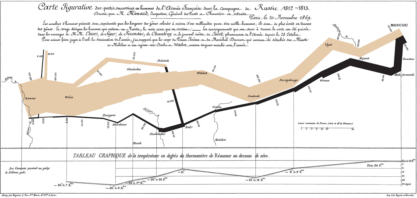
Charles Minard’s map of Napoleon’s Russian campaign in 1812-1813.
The Minard visual handles time well because the temperature chart matches single points on the map; each temperature value was taken at a specific location. Showing time changes in line or area features, such as roads or counties, is harder and is usually handled through symbology. In 1944, the US Army Corps of Engineers created a map showing historical meanders in the Mississippi River. The meanders are not discrete points but cover wide areas. Thus, past river channels are shown in different colors and hatch patterns. While the overlapping meanders are visually complex, the user can easily see the different river channels. Furthermore, the meanders are ‘stacked’ chronologically, so the older meanders seem to recede into the map’s background, similar to how they occur further back in time.
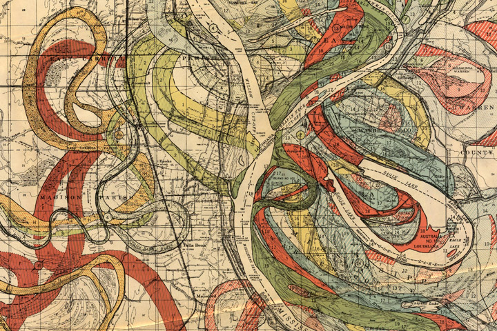
Inset from Geological Investigation of the Alluvial Valley of the Lower Mississippi River.
Another way to handle time is to simply make several maps of the same features, but showing data from different times. In other words, a temporal data set is “sliced” into data sets for a specific time period. The viewer can scan the multiple maps and make visual comparisons. For example, the Southern Research Station of the US Forest Service published a “report card” in 2011 for Forest Sustainability in western North Carolina. To show different land users over time, small maps were generated by county for three years. Undeveloped land is colored green and developed land is tan. Putting these small maps side by side shows the viewer a powerful story of increasing development as the tan expands dramatically. The only drawback is that the viewer must mentally manipulate the maps to track a specific location.
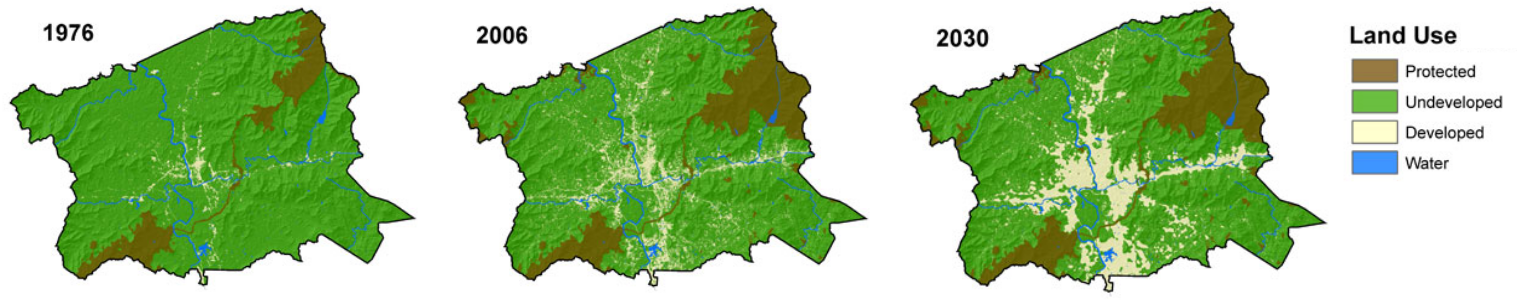
Land Use change over time for Buncombe County, NC
GIS and Time
The previous map examples prove that techniques exist to successfully show time on maps. However, such techniques are not widespread. Furthermore, in the era of “big data” and the “Internet of Things”, showing time is even more important. Consider two examples. First, imagine a shipment of 100 hazardous waste containers being delivered on a truck from a manufacturing facility to a disposal site. The truck has a GPS unit which transmits its location during the drive. Once at the disposal site, each container’s active RFID tag with a GPS receiver tracks the container’s location as it proceeds through any decontamination, disposal, and decommission activities. The locations of the truck and all containers have both a spatial and a temporal component. How can you map the location of all containers over time?
As a second example, consider mobile data collection instruments deployed near a facility to check for possible contamination in the air. Each instrument has a GPS so it can record its location when the instrument is periodically relocated. Each instrument also has various sensors that check every minute for chemical levels in the air plus wind speed and temperature. All these data points are sent back to a central data repository. How would you map chemical levels over time when both the chemical levels and the instrument locations are changing?
In both cases, traditional flat maps would not be very useful given the large amounts of data that are involved. With the advent of GIS, though, all the power of modern computers can be leveraged. GIS has a powerful tool for showing time: animation. Animation is similar to the small “time slice” maps mentioned above, but more powerful because the slices can be shown consecutively like a movie, and many more time slices can be created. Furthermore, the viewer no longer has to mentally stack maps, and it is easier to see changes over time at specific locations.
Locus has adopted animation in its GIS+ solution, which lets a user use a “time slider” to animate chemical concentrations over time. When a user displays EIM data on the GIS+ map, the user can decide to create “time slices” based on a selected date field. The slices can be by century, decade, year, month, week or day, and show the maximum concentration over that time period. Once the slices are created, the user can step through them manually or run them in movie mode.
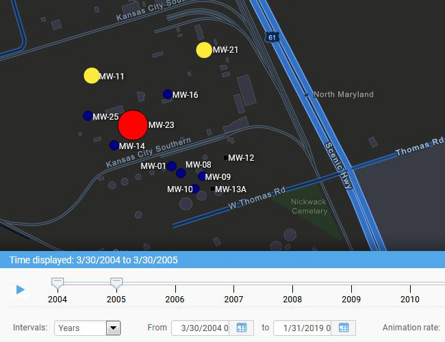
To use the time slider, the user must first construct a query using the Locus EIM application. The user can then export the query results to the GIS+ using the time slider option. As an example, consider an EIM query for all benzene concentrations sampled in a facility’s monitoring wells since 2004. Once the results are sent to the GIS+, the time slider control might look like what is shown here. The time slices are by year with the displayed slice for 3/30/2004 to 3/30/2005. The user can hit play to display the time slices one year at a time, or can manually move the slider markers to display any desired time period.

Locus GIS+ time slider
Here is an example of a time slice displayed in the GIS+. The benzene results are mapped at each location with a circle symbol. The benzene concentrations are grouped into six numerical ranges that map to different circle sizes and colors; for example, the highest range is from 6,400 to 8,620 µg/L. The size and color of each circle reflect the concentration value, with higher values corresponding to larger circles and yellow, orange or red colors. Lower values are shown with smaller circles and green, blue, or purple colors. Black squares indicate locations where benzene results were below the chemical detection limit for the laboratory. Each mapped concentration is assigned to the appropriate numerical range, which in turn determines the circle size and color. This first time slice for 2004-2005 shows one very large red “hot spot” indicating the highest concentration class, two yellow spots, and several blue spots, plus a few non-detects.
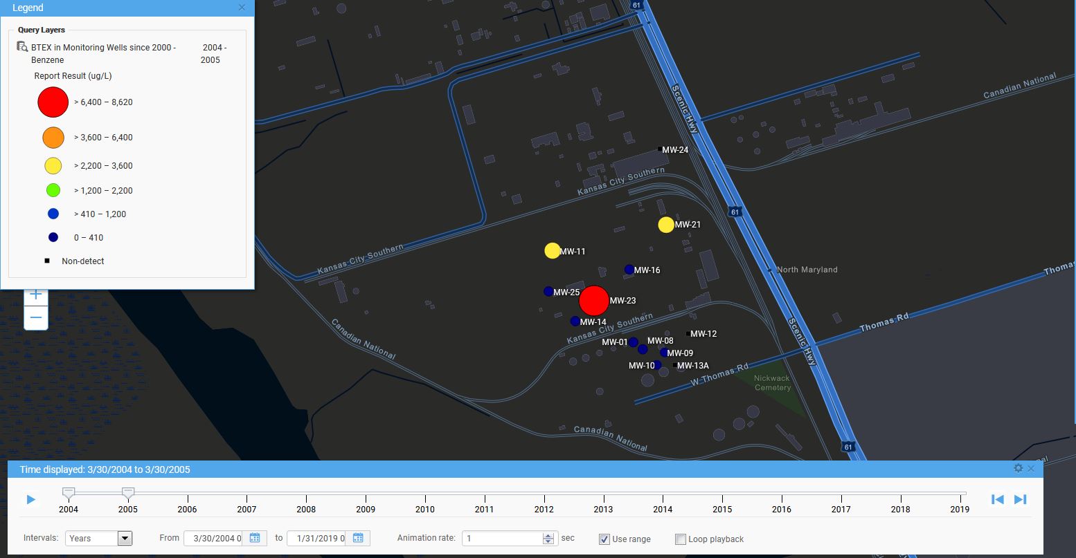
Time slice for a year for a Locus GIS+ query
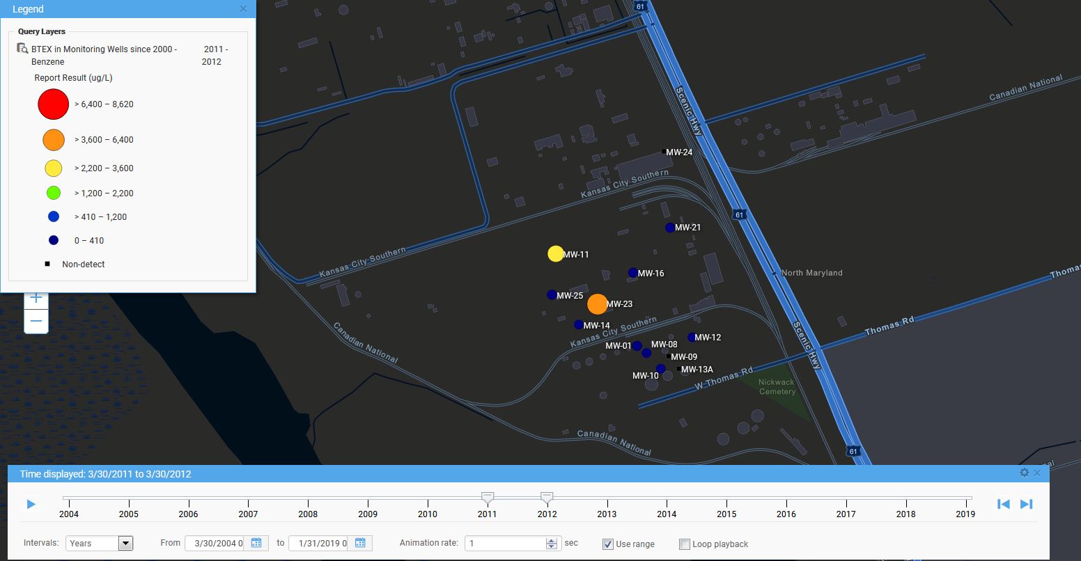
Starting the time slider runs through the yearly time slices. As time passes in this example, hot spots come and go, with a general downward trend towards no benzene detections. In the last year, 2018-2019, there is a slight increase in concentrations. Watching the changing concentrations over time presents a clear picture of how benzene is manifesting in the groundwater wells at the site.
GIS+ time slider in action
While displaying time in maps has always been a challenge, the use of automation in GIS lets users get a better understanding of temporal trends in their spatial data. Locus continues to bring new analysis tools to their GIS+ system to support time data in their environmental applications.
Time slice for a Locus GIS+ query
Interested in Locus’ GIS solutions?
Locus GIS+ features all of the functionality you love in EIM’s classic Google Maps GIS for environmental management—integrated with the powerful cartography, interoperability, & smart-mapping features of Esri’s ArcGIS platform!
Learn more about Locus’ GIS solutions.
Dr. Pierce manages a team of programmers tasked with development and implementation of Locus’ EIM application, which lets users manage their environmental data in the cloud using Software-as-a-Service technology. Dr. Pierce is also directly responsible for research and development of Locus’ GIS (geographic information systems) and visualization tools for mapping analytical and subsurface data. Dr. Pierce earned his GIS Professional (GISP) certification in 2010.